User:Imagico/Coastline Mapping from Landsat Scenes
This tutorial describes the basic workflow of mapping coastlines from Landsat imagery by creating a raster land/water mask and vectorizing it. This is more often more efficient than manually tracing the coastline in the editor and it also ensures some uniformity in the data. It is particularly useful for replacing/supplementing PGS data in areas were high resolution aerial images are not available or not suited for coastline mapping.
Warning
The process described here can also be used to produce data for imports which are subject to the Mechanical Edit Policy. To not fall under the regulations of this policy when mapping with this approach you need to make sure you verify every feature you generate against the source imagery used and you carefully merge the generated data with existing data from the OSM database and make sure no better data (more accurate or more up-to-date) is removed and the coastline data is consistent after your edit (see natural=coastline for the basics).
In the end it requires as much diligence and knowledge of the geography to map an area in good quality using this approach as it does when using conventional tracing techniques.
Required tools
The workflow described here requires the following tools:
- GDAL/OGR with python bindings
- potrace version 1.11
- The geotiff2shp script
- The ls2rgb.py script
- The gdalcopyproj.py script which is part of the GDAL package but normally not installed. You can get it for example from [1]
- Optional: for pansharpening the images: the gdal_landsat_pansharp program from dans-gdal-scripts.
- An image editor of your choice like GIMP
- Not required but very useful for looking at the various geodata files is QGIS
- JOSM with opendata plugin
On Windows you will probably also need various other stuff not available there by default.
Process description
Getting satellite imagery
In principle you can use any kind of satellite or aerial imagery but this method works best with data from the near infrared spectrum where water and land have a good contrast. This tutorial will be based on Landsat 8 data.
Landsat images are freely available but to download up-to-date scenes you need to register an account with the USGS. A few Landsat 8 scenes and a lot of older Landsat 7 data (including what is used as source for PGS) is available without registration from the GLFC
The process of downloading from the USGS is described in detail in this tutorial
A single landsat scene is a 800MB-1GB gzipped tar archive that unpacks to about 2GB. In the following i will use scene LC81900182013233LGN00 as example.
Processing the Landsat data
After unpacking by running
tar xvfz LC81900182013233LGN00.tar.gz
you get a number of tiff files and a metadata text file:
LC81900182013233LGN00_B1.TIF
LC81900182013233LGN00_B2.TIF
LC81900182013233LGN00_B3.TIF
LC81900182013233LGN00_B4.TIF
LC81900182013233LGN00_B5.TIF
LC81900182013233LGN00_B6.TIF
LC81900182013233LGN00_B7.TIF
LC81900182013233LGN00_B8.TIF
LC81900182013233LGN00_B9.TIF
LC81900182013233LGN00_B10.TIF
LC81900182013233LGN00_B11.TIF
LC81900182013233LGN00_BQA.TIF
LC81900182013233LGN00_MTL.txt
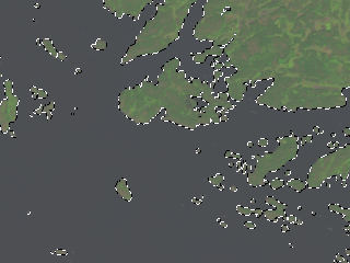
The data comes in separate files for each of the spectral channels. As already mentioned the infrared channels are most useful for distinguishing water from land. In principle you can use any channel combination you want but mapping channels 6, 5 and 4 to red, green and blue is a good start. This will lead to bare ground in reddish tones, vegetation in green, snow/ice in blue and clear water in very dark blue.
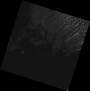
raw channel 6 image
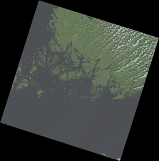
6/5/3 channel combination with gamma correction and scaling


To simplify assembling the channels you can use the ls2rgb.py script that assembles three single channel 16 bit images to a 3 channel rgb 8 bit image and allows performing basic value scaling (i.e. 'exposure control') and gamma correction. So for the 6/5/4 channel combination you run:
ls2rgb.py -s 1.2 -g 2.0 LC81900182013233LGN00_B6.TIF LC81900182013233LGN00_B5.TIF LC81900182013233LGN00_B4.TIF LC81900182013233LGN00_654.tif
The aim here is not to produce a pretty looking image but to clearly see the difference between water and land.
Optional: pansharpening the image
This additional step is optional, you can work through this tutorial without it. Following this steps requires building the gdal_landsat_pansharp tool (see link above) which requires a working C++ toolchain including the boost libraries and autoconf/automake.
What is called pansharpening is the use of the high spatial resolution panchromatic channel data of a satellite to supplement the lower spatial resolution multispectral data. There are various methods to do this and the mentioned tool implements one of them. Using
gdal_landsat_pansharp -rgb LC81900182013233LGN00_B6.TIF -rgb LC81900182013233LGN00_B5.TIF -rgb LC81900182013233LGN00_B4.TIF \
    -lum LC81900182013233LGN00_B2.TIF 0.1 -lum LC81900182013233LGN00_B3.TIF 0.5 -lum LC81900182013233LGN00_B4.TIF 0.4 \
    -pan LC81900182013233LGN00_B8.TIF -ndv 0 -o LC81900182013233LGN00_654p.tif
you can generate a pansharpened version of the 6/5/4 channel combination. Note the factors used are different from the ones mentioned in the tools documentation since Landsat 8 has a different spectral characteristic than Landsat 7 (in fact the Landsat 7 data would be better suited for this particular application). Note the numbers are just an educated guess but the exact values do not matter that much unless there are very strong colors in the scene.
The resulting 3-channel-image is in linear 16 bit form and you can use the ls2rgb.py to produce a gamma corrected 8 bit version:
ls2rgb.py -s 1.2 -g 2.0 LC81900182013233LGN00_654p.tif LC81900182013233LGN00_654p.tif LC81900182013233LGN00_654p.tif LC81900182013233LGN00_654g.tif
(yes, that's three times the same file name, the script automatically chooses the channels). Below you can see the difference in resolution. In the following you can use LC81900182013233LGN00_654g.tif instead of LC81900182013233LGN00_654.tif in case you did the pansharpening.
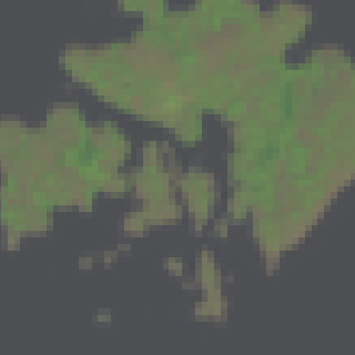
normal multispectral image
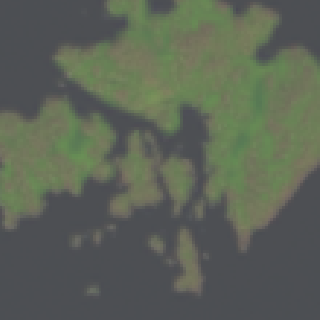
pansharpened image


Generating the land/water mask
next you need to generate a land/water mask from the image. For this you load the image into your favorite image editor and mask the water just like you would in a photo for example to replace the background. The scene chosen as example here makes this very easy since it has nearly no clouds across the coastline, hardly any turbidity in the water and a high sun position combined with fairly flat terrain so no shadowing. Normally masking the water is much more hand work, using the fuzzy select tool in combination with a brush is often a good approach. But here you can essentially use the select by color tool on an average water area to pretty reliably select all water in the scene with a single click (in GIMP for example using a threshold of 15). You will notice however that in the upper right of the scene the cloud shadows are then masked as water and clouds over water turn up als land (which does not matter since we won't use those parts of the scene anyway). But it is easy to miss a small patch of clouds so keep in mind the warning above - you need to verify the data you produce before you can consider uploading it to OSM. After selecting the water just fill the whole selection with black, invert the selection and fill the rest with white (for the next steps to work as they are described land should be white and water should be black - no gray pixels).
selecting the water areas in GIMP
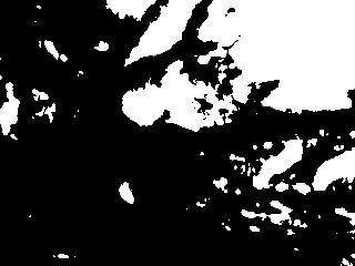
mask created from selection


Once finished save the mask as a grayscale image in tiff format. Since GIMP and other imaging programs are unaware of the geographic coordinates stored in the tiff file you need to transfer those from the original data using
gdalcopyproj.py LC81900182013233LGN00_B6.TIF LC81900182013233LGN00_mask.tif
or (in case your mask is created from the pansharpened image):
gdalcopyproj.py LC81900182013233LGN00_B8.TIF LC81900182013233LGN00_mask.tif
Note for this to work it is of course important that the mask image is exactly the same size as the original image. So no cropping and resizing inside GIMP.
Usually the area you will actually want to map is smaller than the whole Landsat scene so before the next step we are going to crop it:
gdalwarp -te 490000 6620000 540000 6670000 LC81900182013233LGN00_mask.tif LC81900182013233LGN00_mask_clip.tif
These coordinates are in UTM projection (the coordinate system the Landsat scene comes in). The easiest way to find out the coordinates of the area you want is to load the image into QGIS. If the scene is too large to comfortably work on in the imaging program (this might be the case, especially with the pansharpened version) you can also do the cropping before creating the mask.
full scene as land/water mask
cropped to the area of interest


Vectorizing the mask
Once you have produced an accurate land/water mask as described above you can vectorize it using potrace. Vectorization here means producing a polygon vector geometry from the raster mask data. potrace itself does not read the coordinate metadata in the raster file but the geotiff2shp converts this information into the appropriate potrace options and also converts the GeoJSON output into a shapefile:
geotiff2shp.sh LC81900182013233LGN00_mask_clip.tif LC81900182013233LGN00_mask.shp
A look at the resulting polygon data reveals the vectorization performed by potrace produces overly dense lines in some parts with significantly more nodes than necessary. You can simplify this using ogr2ogr. At the same time we can reproject the data from UTM coordinates to the latitude/longitude coordinates used by Openstreetmap:
ogr2ogr -simplify 2 -t_srs "EPSG:4326" LC81900182013233LGN00_mask2.shp LC81900182013233LGN00_mask.shp
Note with ogr2ogr the first file is the output and the second file is the input data. The amount of simplification is a matter of choice - a value of 2m is fairly reasonable for pansharpened landsat data.
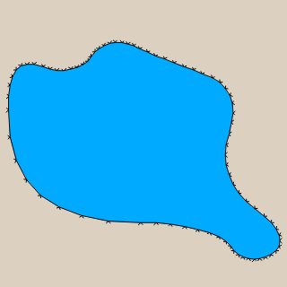
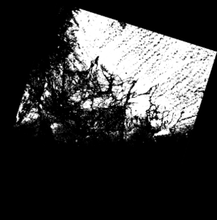
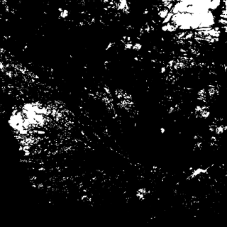
original potrace output in QGIS
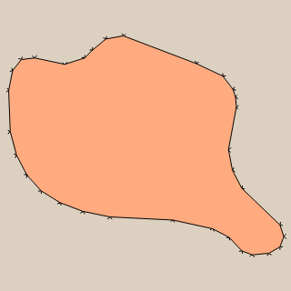
after line simplification


Aligning and merging the data into the map
We can now load the resulting file into JOSM using the opendata plugin. When we do that we can see there is a significant offset to the high resolution Bing images. Landsat scenes can vary greatly in positional accuracy depending on the location on earth. An option can be provided to the geotiff2shp for correcting simple constant offsets. Using
geotiff2shp.sh LC81900182013233LGN00_mask_clip.tif LC81900182013233LGN00_mask.shp "" "" "30.0:20.0"
will approximately compensate the offset here. The offset of about 35m seen here is about average in this area but be aware it can also be significantly larger. Same applies for existing PGS based coastline data in OSM which is also based on Landsat images with a similar positional accuracy. Note Bing images should be checked and corrected for offsets before using them as reference for this purpose - aligning satellite images based on equally unaligned aerial images or PGS data is pointless. Best is to use quality GPS data where available.
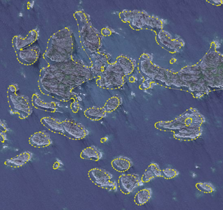
vectorized mask in JOSM with offset
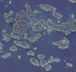
with offset corrected


Next thing you should do before merging with existing OSM data is reversing all ways (select all and press R in JOSM) since processed the way described they have the wrong orientation for coastlines. After that you can load existing data from OSM into a separate layer and start merging features from your newly vectorized coastline one by one with the existing data.
When you upload the data to OSM make sure to include the Landsat scene ID and the method used in the changeset tags/comment.
Closing Remarks
A few words on accuracy
The coastline data produced using the described technique provides similar amounts of detail, i.e. capability to resolve for example small islands, when compared to good quality PGS data. In extreme cases when using Landsat 8 data the lack of infrared sensitivity in the panchromatic channel can lead to a slight disadvantage. More importantly there are a number of serious advantages of this method though:
- PGS being a ready-made data set is only as good as the images it is produced from and those are hampered with significant cloud cover in some areas.
- The method described here does not produce the unnatural sharp corners known from PGS data.
- With a properly generated mask as basis there is significantly better quantitative accuracy compared to PGS, for example the sizes of small islands tends to be much more reliable than in case of PGS.
- You can use up-to-date Landsat imagery as a basis while PGS source data is more than 10 years old.
- By properly aligning the source imagery you can achieve a much better positional accuracy than with PGS data.
The sample area chosen for this tutorial is also covered by high resolution Bing imagery which allows comparing the resolution. It can be seen that small bays and narrows between the skerries are not resolved. This is partly because the masking i used is somewhat land biased meaning there is more focus on not missing small islands than on not missing small narrows between them. More sophisticated processing for mask production could reduce that effect a bit.
Where to go from here
This tutorial describes only the basics, there are a lot of way this technique can be extended:
- Instead of loading the resulting shapefile into JOSM and applying all tags by hand you can also use one of the import tools (see Import/Shapefile) to convert the data into OSM format and apply the tags needed. But keep in mind the warning above and make sure that if you end up doing a true import you follow the correct procedures.
- You can produce the land/water mask using several Landsat scenes which is especially useful if every single one of them contains clouds in some parts or if you use newer Landsat 7 images with SLC gaps. Best is to crop them to the same extent and projection using GDAL tools and then load them as separate layers into the imaging program.
- Of course in principle you can use this technique to map other things than the coastline. Obviously you can do lakes in exactly the same way (the mask generated in the example above already includes those) but you can also identify and map vegetation cover or other features that can reliably be identified on the source image. But since potrace only deals with black/white images you will have to perform more sophisticated post processing.
- To use this method for other imagery than Landsat 8 you will need to adapt the workflow a bit. In particular when processing 8 bit images with ls2rgb.py you will need to adjust the value scaling to 1/256.
Areas of possible application
The most useful areas for application of this method are of course were no high resolution data is available. A few examples:
- Indonesian islands and Landsat scene for possible use
- Pacific coast of Panama and Landsat scene for possible use
- Kamchatka east coast and Landsat scene for possible use
- Chile coast and Landsat scene for possible use - beware of shadows here since this is a winter scene.
A few more examples - for some of these areas also high resolution Bing imagery is available:
- Northern Australia and Landsat scene for possible use - current OSM data here is not PGS but a fairly coarse local source by the way.
- Sulawesi and Landsat scene for possible use - currently partly with node distances of several km due to cloud cover.
- Myanmar and Landsat scene for possible use - large areas of mangrove forest there are mapped as sea.
- Wolga delta and Landsat scene for possible use
- Southern Alaska and Landsat scene for possible use - Lakes are missing here too.
What about scanaerial?
Scanaerial is a tool for automatically detecting areas in satellite/aerial images which is somewhat similar to the technique described here. But there are a few important differences:
- Scanaerial relies on tiles/wms services in JOSM which are usually not so good for detecting water surfaces.
- While there are a few options that can be adjusted in the configuration file there is not much control over the actual feature detection process. As a result you usually get either too much of the image classified as water or too little.
- The polygons produced have unnatural sharp corners similar to the PGS.
- Scanaerial requires manually selecting every waterbody and is not really suited for the coastline.
Links
- GDAL/OGR - library including various tools for raster and vector geodata processing
- potrace - vectorization program with GeoJSON output in version 1.11
- geotiff2shp - wrapper script for potrace
- ls2rgb.py - assembling Landsat channels to rgb images
- gdalcopyproj.py download - also included in the GDAL source package but not installed by default.
- dans-gdal-scripts - including gdal_landsat_pansharp and some background information
- Landsat at the USGS
- EarthExplorer - USGS tool for searching and downloading Landsat scenes
- GLOVIS - another Java based USGS tool for searching and downloading Landsat scenes
- Tracing Landsat 8 for OpenStreetMap on the Mapbox blog
- some info on the different spectral channels of Landsat